Scope
How text (and images) become vectors, and how you search billions of them fast. Embedding model selection by task not leaderboard, similarity metrics and their silent bugs, the ANN index trade-space (HNSW / IVF-PQ / ScaNN), the vector-DB landscape, hybrid search + Reciprocal Rank Fusion, and the 2026 cost levers — Matryoshka truncation, int8/binary quantization, multi-vector late interaction. This is the retrieval substrate under RAG. For the end-to-end retrieve→rerank→generate pipeline see 07 - RAG; for shipping the index see 17 - Deployment & Serving.
Related: Gen AI Engineer, 07 - RAG, 17 - Deployment & Serving
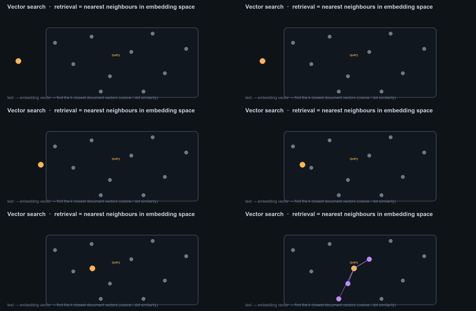
Query and documents map into the same vector space; nearest neighbours by similarity are the “relevant” results.
1. The concept: meaning as geometry
An embedding model maps text into a fixed-length vector (e.g. 1024 floats) such that semantically similar text lands close together. “Refund policy” and “how do I get my money back” sit near each other even with zero shared words — that is the whole point, and the reason embeddings beat keyword search on paraphrase and synonym.
Retrieval then becomes a geometry problem: embed the query, find the corpus vectors nearest to it. The catch is scale — brute-force comparison against millions of vectors is too slow, so we use Approximate Nearest Neighbor (ANN) indexes (§6) that trade a little recall for orders-of-magnitude speed.
Mental model
Embedding = lossy compression of meaning into coordinates. Everything downstream (metric, index, quantization) is a trade between how much of that meaning you keep and how cheap/fast search becomes.
2. Choosing an embedding model: task, not MTEB rank
The most common mistake is picking whatever tops the MTEB leaderboard. MTEB is an aggregate across dozens of tasks and languages; your job is one task on your data. A model ranked #4 overall can beat #1 on your domain.
Current families to know (mid-2026):
| Model family | Type | Notes |
|---|---|---|
| OpenAI text-embedding-3 (small/large) | API | strong general baseline; text-embedding-3-large still tops MTEB in early 2026; supports dimension truncation; cheap (small ≈ $0.02/M tokens) |
| Cohere embed-v4 | API | separate search_document / search_query input types (asymmetric); multimodal; tight rerank-v3 integration |
| Voyage (voyage-3-large, voyage-4) | API | retrieval-optimized; voyage-4 (Jan 2026) uses Mixture-of-Experts; strong on their RTEB retrieval benchmark; priciest (large ≈ $0.18/M) |
| Qwen3-Embedding (0.6B/4B/8B) | open | topped MTEB-multilingual mid-2025; 32k context, 100+ langs; sizes give cost/quality dial |
| BGE-M3 | open | MIT license; one model does dense + sparse + multi-vector; 100+ langs; ~8k context |
| E5 / NV-Embed | open | strong instruction-tuned dense encoders; NV-Embed-v2 a frequent open SOTA reference |
MTEB ≠ your domain
Benchmark candidates on your own labeled queries, measuring the metric you actually serve (Recall@k / NDCG@k). Legal, medical, code, and multilingual corpora routinely reorder the leaderboard. A 50-100 query gold set built in an afternoon beats any public chart.
Asymmetric (query vs document) models
Some models (Cohere embed-v4, E5, BGE) embed queries and documents differently — a short question and a long passage are not symmetric. Use the prescribed prefix / input-type or you silently lose recall.
3. Bi-encoder vs cross-encoder
Two architectures, two jobs — and the source of the standard two-stage retrieval pattern:
| Bi-encoder | Cross-encoder | |
|---|---|---|
| How | encodes query and doc separately into vectors; compare with a metric | feeds query+doc together through one transformer, outputs a relevance score |
| Speed | precompute all doc vectors once; query is one forward pass + ANN lookup | must run the model on every (query, doc) pair at query time |
| Quality | good | better — full cross-attention sees interactions |
| Role | retrieval (search millions) | reranking (re-score the top ~50-100) |
The production pattern: bi-encoder + ANN to fetch candidates cheaply, then a cross-encoder reranker to reorder the shortlist. You cannot use a cross-encoder for first-stage search — it does not produce a reusable vector, so there is nothing to index. (Reranking detail lives in 07 - RAG.)
4. Dimensionality vs cost
Higher dimensions can capture more nuance but cost linearly more on storage, RAM, and per-comparison compute, and they raise index build time. A 3072-dim float32 vector is 12 KB; 100M of them is ~1.2 TB before any index overhead. Dimensionality is a first-order cost lever, which is exactly why Matryoshka (§9) and quantization (§10) matter.
5. Similarity metrics — and the silent mismatch bug
| Metric | Measures | When |
|---|---|---|
| Cosine | angle (direction), ignores magnitude | default for most text embeddings |
| Dot product | direction and magnitude | only correct if vectors are normalized (then ≡ cosine), or if the model was trained for raw dot product |
| Euclidean (L2) | straight-line distance | some models/clustering; equivalent to cosine on normalized vectors |
The metric / normalization mismatch — a silent recall killer
If you index with the wrong metric for how the model was trained, you get no error — just quietly degraded results that look like a “bad model.” Two classic forms:
- Using dot product on un-normalized vectors when the model expects cosine → longer documents dominate purely because they have bigger magnitude.
- Switching the DB’s distance metric without re-normalizing.
Always use the metric the model card specifies, and normalize if it says to. This bug survives code review because it throws nothing.
6. ANN indexes: the recall / latency / memory / build trade-space
Brute force (“Flat”) is exact and is the right answer below ~100k vectors. Past that you pick an ANN index, and every index is a point in a four-way trade-off: recall, query latency, memory, build cost.
| Index | Recall | Latency | Memory | Build | Use when |
|---|---|---|---|---|---|
| Flat (brute force) | 100% | high | high | none | small corpus, exact baseline |
| HNSW (graph) | 95-99% | very low | high | medium | the default 100k-10M; high recall, low latency, frequent updates — if RAM allows |
| IVF-PQ (cluster + product quantization) | 90-95% | medium | low | high | huge corpora (10M-1B+) where RAM is the bottleneck |
| ScaNN (Google) | 95-99% | low | medium | medium | middle ground; strong at scale on Google stacks |
How they work, briefly:
- HNSW builds a multi-layer proximity graph and greedily hops toward the query. Tune
ef_search(higher = more recall, more latency) andM(graph degree, memory). Fast and update-friendly but the graph lives in RAM. - IVF partitions vectors into clusters; at query time you only scan the
nprobenearest clusters. PQ then compresses each vector into a few bytes of cluster codes, slashing memory at some recall cost. IVF needs a training step on a sample, hence higher build cost. - ScaNN combines partitioning with an anisotropic quantization tuned for inner-product, giving HNSW-class recall at lower memory.
Pick by your binding constraint
RAM-rich, need top recall + low latency, data churns → HNSW. Memory-bound at 100M+ vectors → IVF-PQ (or IVF + RaBitQ). Under ~100k → just use Flat and stop optimizing.
7. Vector DB landscape
Choose by scale, filtering needs, and ops appetite — not hype.
| DB | Sweet spot | Notes |
|---|---|---|
| pgvector | < ~5M vectors | lives inside your existing Postgres — one system, transactions, joins. Start here if you already run Postgres. |
| Qdrant | up to hundreds of millions / single node | Rust engine, best-in-class filtered search (ACORN keeps filters fast inside HNSW traversal); strong perf-per-dollar |
| Weaviate | mid-large + hybrid | native BM25 + vector fusion built in, so you don’t run two search systems |
| Milvus | 1B+ / GPU | distributed architecture, GPU-accelerated indexing; reach for it at extreme scale |
| Pinecone | managed, zero-ops | fully hosted, fast at scale; you pay to not run infra |
Don't reach for a dedicated vector DB too early
If you have Postgres and a few million vectors, pgvector avoids an entire new system to operate, secure, and back up. Migrate when scale, filtering, or hybrid needs actually force it.
8. Hybrid search + Reciprocal Rank Fusion
Dense embeddings miss exact tokens — product SKUs, error codes, rare names, acronyms. Keyword/lexical search (BM25) nails those but misses paraphrase. Hybrid search runs both and fuses the results; reported recall gains are commonly 15-30% over either alone.
Reciprocal Rank Fusion (RRF) is the standard, robust fuser. Each list gives a document at rank r a score 1 / (k + r) (typically k=60), summed across lists:
score(d) = Σ_lists 1 / (k + rank_list(d))
RRF wins because it uses rank, not raw scores — so you never have to normalize incompatible BM25 and cosine scales (a common source of bad fusions). Add a cross-encoder rerank on the fused top-N for the best quality (see 07 - RAG).
9. Matryoshka embeddings (truncatable dimensions)
Matryoshka Representation Learning (MRL) trains so that the most important information is packed into the leading dimensions. You can chop a 1024-dim vector down to 256 (or 128) by simple truncation and keep most of the quality — typically ~2% drop for a large cut. OpenAI text-embedding-3 and many recent models support this.
Why it matters: store the full vector, but search on the truncated prefix for cheap first-pass retrieval, then rerank on full dimensions. One model, multiple cost/quality points, no re-embedding. MRL is orthogonal to quantization — you can truncate and quantize.
10. Quantization: 4× to 32× smaller
Compress the float32 vector itself:
| Scheme | Size vs float32 | Quality retained | Note |
|---|---|---|---|
| int8 scalar | ~4× smaller | ~98-99% | each value → 8-bit int; recall drop often ~1-3% |
| binary | ~32× smaller | ~95-96% | each value → 1 bit; search with Hamming distance, then rerank survivors on full vectors |
| RaBitQ / BBQ | ~32× (binary) | high | theoretically-grounded binary quantization (basis of Elasticsearch/Lucene “Better Binary Quantization”); much better quality than naive binary at the same size |
The standard high-recall recipe
Search fast on binary vectors to get a large candidate pool, then rerank that pool on the full-precision (or int8) vectors. You get ~32× cheaper first-pass search and recover almost all the quality. Quantization stacks with Matryoshka for compounding savings (reported up to ~80% cost reduction, and far more in research pipelines).
11. Multi-vector / late interaction (ColBERT, ColPali)
Single-vector embeddings squash a whole passage into one point — fine, but lossy for long or detailed documents. Late-interaction models keep a vector per token and score by summing each query token’s best match against the document tokens (MaxSim):
- ColBERT — the original token-level late interaction; much higher quality than single-vector on hard retrieval, at the cost of far larger indexes (many vectors per doc).
- ColPali / ColQwen — late interaction over document images: treat a PDF page as image patches (built on PaliGemma / Qwen-VL), retrieving over layout, tables, and figures without OCR or chunking. Strong for visually rich documents.
Trade-off: best-in-class recall, but storage and compute balloon (per-token vectors). Often used as a high-quality reranking stage rather than the primary index.
12. SPLADE (learned sparse)
SPLADE produces a sparse vector over the vocabulary — like BM25, but the model learns term weights and expands to related terms (so “car” can activate “vehicle”). It runs on inverted indexes (cheap, interpretable, exact-match friendly) while capturing some semantics. A practical middle path: keyword-search efficiency with learned recall, and a natural component of hybrid pipelines.
13. Embedding fine-tuning
When an off-the-shelf model underperforms on your domain, fine-tune it on (query, relevant passage) pairs (contrastive / hard-negative training). Big gains on jargon-heavy or niche corpora.
Fine-tuning forks your model
A fine-tuned embedder is a new model version. Every vector in your corpus was produced by the old one — you must re-embed the entire corpus to use it (see §15). Budget the re-embed before you commit.
14. Filtered ANN: pre-filter vs post-filter
Real queries carry metadata constraints (“docs from this tenant, after this date”). Two strategies, both with failure modes:
| Strategy | How | Failure mode |
|---|---|---|
| Post-filter | ANN first, drop non-matching results after | a selective filter can leave too few or zero results — the top-k all got filtered out |
| Pre-filter | restrict the candidate set, then ANN | naive pre-filtering breaks the index’s graph/cluster structure → slow or low recall |
The good systems solve this inside the index: Qdrant’s ACORN keeps HNSW traversal filter-aware so selective filters stay both fast and high-recall. This is a real differentiator when filtering is central — evaluate it on your filter selectivity, not generic benchmarks.
15. ⚠️ Caveats & risk mitigation
- Swapping the embedding model re-embeds the WHOLE corpus. Vectors from model A are incomparable to vectors from model B — different geometry. Changing or fine-tuning the model means re-embedding every document and rebuilding the index. Version the model with the index and the corpus together; treat a model change as a full reindex migration (blue/green the index, backfill, then cut over). This is the single biggest operational gotcha in vector search.
- MTEB ≠ your domain. (§2) Benchmark on your own data. Leaderboards mislead on niche corpora.
- The metric/normalization mismatch is silent. (§5) Wrong metric throws no error, just quietly tanks recall. Match the model card.
- ANN is approximate. “Missing” results may be a recall setting (
ef_search/nprobe), not a bad embedding. Measure Recall@k against a Flat baseline before blaming the model. - Quantization/truncation trade quality. Always re-measure recall on your gold set after enabling int8/binary/MRL — the “~96%” figures are corpus-dependent.
- Embedding inversion is a privacy risk. Embeddings are not anonymized data. Inversion attacks (e.g. Vec2Text) can reconstruct a large fraction of the original text from its vector — research reports up to ~92% of short inputs recovered, including sensitive strings. Treat stored vectors with the same sensitivity as the source text: encrypt at rest, access-control the index, isolate per-tenant. Quantization happens to reduce invertibility somewhat. More in 14 - Safety, Security & Risk.
16. In practice
# Asymmetric embedding + cosine, normalized for a dot-product index
qv = embed(query,   input_type="search_query")     # query-side encoding
dv = embed(passage, input_type="search_document")   # doc-side encoding
# normalize -> dot product == cosine, no silent magnitude bias
qv, dv = normalize(qv), normalize(dv)

# Two-stage retrieval: cheap ANN recall, then expensive rerank
candidates = index.search(qv, top_k=100)             # bi-encoder + HNSW
reranked   = cross_encoder.rank(query, candidates)   # cross-encoder top-100 -> top-10

# Hybrid via RRF: fuse dense + BM25 by RANK, not raw score (k=60)
def rrf(rank_lists, k=60):
    scores = {}
    for lst in rank_lists:                 # [dense_ids, bm25_ids]
        for r, doc in enumerate(lst):
            scores[doc] = scores.get(doc, 0) + 1 / (k + r)
    return sorted(scores, key=scores.get, reverse=True)
Defaults that travel well: HNSW + cosine on normalized vectors, hybrid (dense + BM25) fused with RRF, cross-encoder rerank on the top-100, int8 quantization once you outgrow RAM. Benchmark every choice on your own gold set.
Sources
- Qwen3 Embedding (arXiv 2506.05176)
- Qwen3-Embedding — GitHub
- The Best Open-Source Embedding Models in 2026 — BentoML
- Voyage 3.5 vs OpenAI vs Cohere Embedding Models 2026
- Best Embedding Models 2025: MTEB Scores & Leaderboard — Ailog
- ANN Index Types: When to Choose Flat, HNSW, IVF, or IVF-PQ
- Understanding IVF vs HNSW — Milvus Blog
- Binary and Scalar Embedding Quantization — Hugging Face
- Better Binary Quantization (BBQ / RaBitQ) — Elasticsearch Labs
- Combining Matryoshka with Binary Quantization — Vespa Blog
- Late Interaction Retrieval: ColBERT, ColPali, ColQwen — Weaviate
- Production RAG: Hybrid Search + Re-Ranking (ColBERT, SPLADE)
- pgvector vs Pinecone vs Qdrant vs Weaviate (2026)
- Vec2Text: Inverting Text Embeddings
- Rethinking the Privacy of Text Embeddings (arXiv 2507.07700)